Your Neural Network is Secretly a Kernel Machine
Arunav Gupta, Rohit Mishra, Mehdi Bouassami William Luu
Introduction
Neural networks have been very successful at solving problems of scientific and technological nature. However, our understanding of the theory that explains how they work has been improving slowly compared their practical advancements. By understanding what underlying mechanics make these systems work, we can drastically improve neural networks’ performances.
Our research focuses on investigating essential mechanisms behind feature learning in neural networks that are fully connected to construct a new type of machines called Recursive Feature Machines (RFMs). RFMs ustilize kernels to combine linear separation and feature learning into an iterative process. Our findings are very interesting for the field of machine learning as we noticed that RFMs outperform a lot of classical deep learning networks.
In this project, we started by studying kernel methods which are a type of algorithm that facilitate the transformation of input data into a different dimensional space. We then understood the basics of RFMs and tested their performance on a scaling test and on text prediction. For the scaling test, we compared MSEs of RFMs and a basic Laplacian kernel and for the text generation, we performed a “few-shot next character” prediction problem. We then compared bleu scores and perplexities of RFMs, N-gram and Laplacian kernel.
This project was highly motivated by the popularity of openAI. The usefulness of ChatGPT is impressive and studying text prediction with different neural network models is of actuality.
In summary, we’re investigating why large parameter models perform better, comparing kernel methods to neural networks and recursive feature machines on text datasets, and analyzing the theory behind recursive kernel machines.
What Do Kernels Look Like?
Kernels take the following form:
\[K(x, z) = \exp\left(\frac{-|x-z|L}{σ}\right)\]Where L represents the distance norm and σ the kernel width. L = 1 for the Laplacian Kernel and L = 2 for the Gaussian kernel.
In order to train a kernel, the following equation has to be solved for \(\hat{\alpha}\):
\[\hat{\alpha} = yK(X, X)^{-1}\]To make predictions, use the following equation:
\[\hat{y}(x) = \hat{\alpha}K(X, x)\]What Are Recursive Feature Machines?
RFMs have the following form:
\(K(x, z) = \exp\left(\frac{-|x-z|M}{σ}\right)\)
Where \(|x-z|M := \sqrt{(x-z)^{T}(x-z)}\)
Thus, we can calculate the gradient as follow:
\[\nabla K_{M}(x, z) = \frac{Mx - Mz}{σ|x - z|M}K(x, z)\]How To Train an RFM?
First, let d be the number of features and let \(M := I_{dxd}\) (1)
Then use M to train a kernel \(K_{M}\) (2)
Update M as follow: \(M = \frac{1}{n}\sum_{x \in X}\nabla f(x) \nabla f(x)^{T}\) where \(\nabla f(x) = \alpha \nabla K_{M}(X, x)\) (3)
Finally, cross-validate and repeat 2-4 until convergence (4)
What Are The Benefits of RFMs?
RFMs have a remarkable ability to outperform several neural networks in text classification, as the results section will demonstrate later on. Additionally, RFMs use sparse matrices, making them more data-efficient than other methods. Interestingly, M also converges to the same weights as a learned DNN does on vision tasks.
Our Dataset
Our approach involved using RFMs to predict the next word in a text dataset. To accomplish this, we utilized a PDF version of George Orwell’s 1984 and extracted the raw words from it. We constructed a vocabulary of 50 alphanumeric characters and tokenized the text accordingly. Next, we encoded the characters in a one-hot format and obtained a matrix with dimensions N (number of samples) by 64 (token size) by 50 (vocabulary size). We then compared the performance of our RFM model to that of bigram/trigram models, as well as the Laplacian kernel.
Results
Scaling Test
Before testing the model on text prediction, let’s first look at how the performance of an RFM scales with the model and feature size. In order to do so, we generated 1000 random datapoints \(x_{i} \in R^{d} \rightarrow X\) and used the following target function: \(f(x) = 5x_1^3 + 10x_2^2 + 2x_3\) We then train an RFM and Laplacian Kernel (“Baseline”) and get the test MSE. The results are shown below
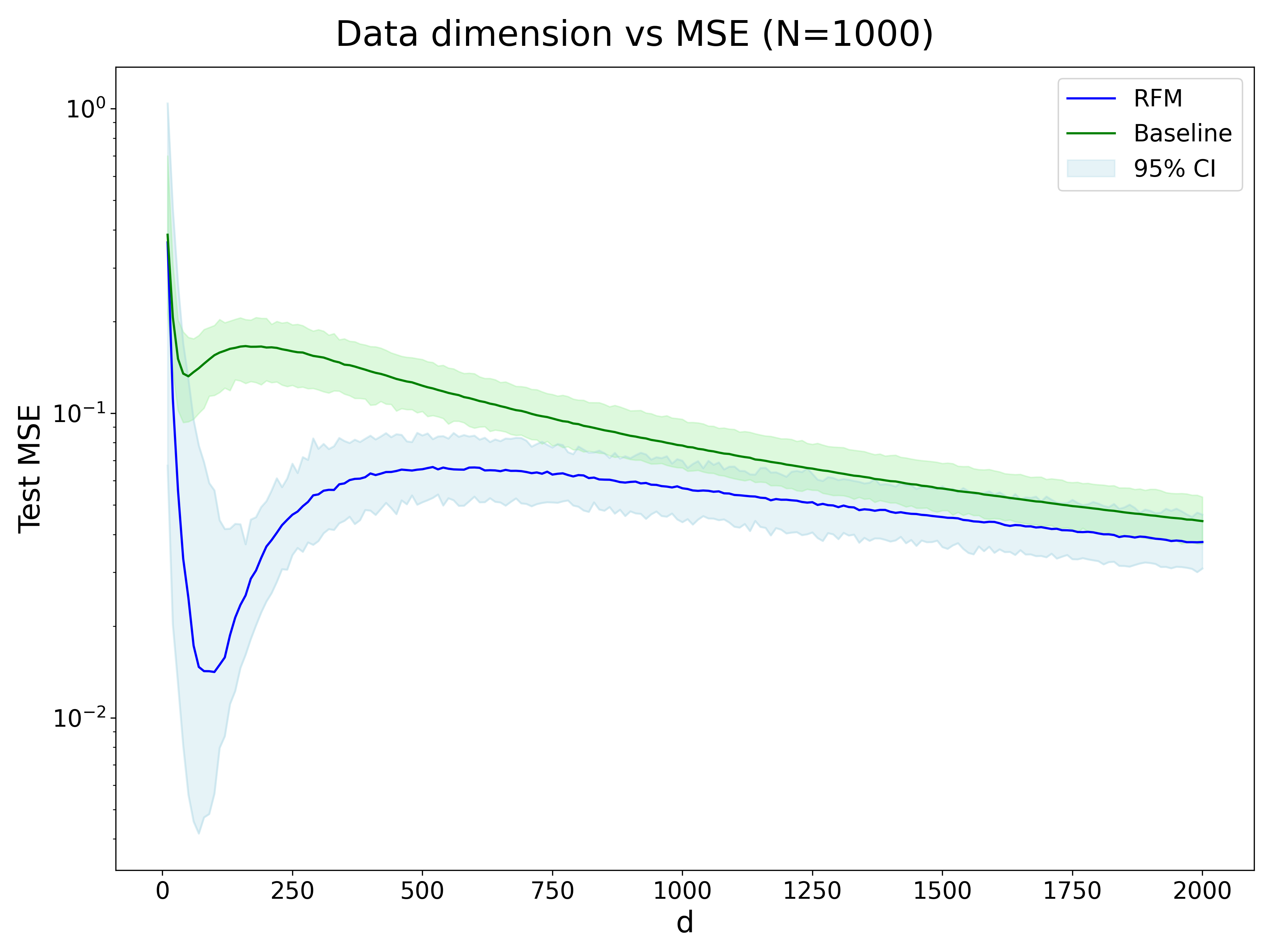
We see that the RFM performs better than the baseline (Laplacian Kernel) when d is between 10 and 200. After that, the MSEs of both models are very similar.
Text Prediction
Now, let’s test the RFM model on the 1984 dataset and see how well it can perform on a few-shot next character prediction problem. In order to have a good idea of how powerful the RFM method is, we compare its performance to traditional methods N-grams and kernels. Here are the results:
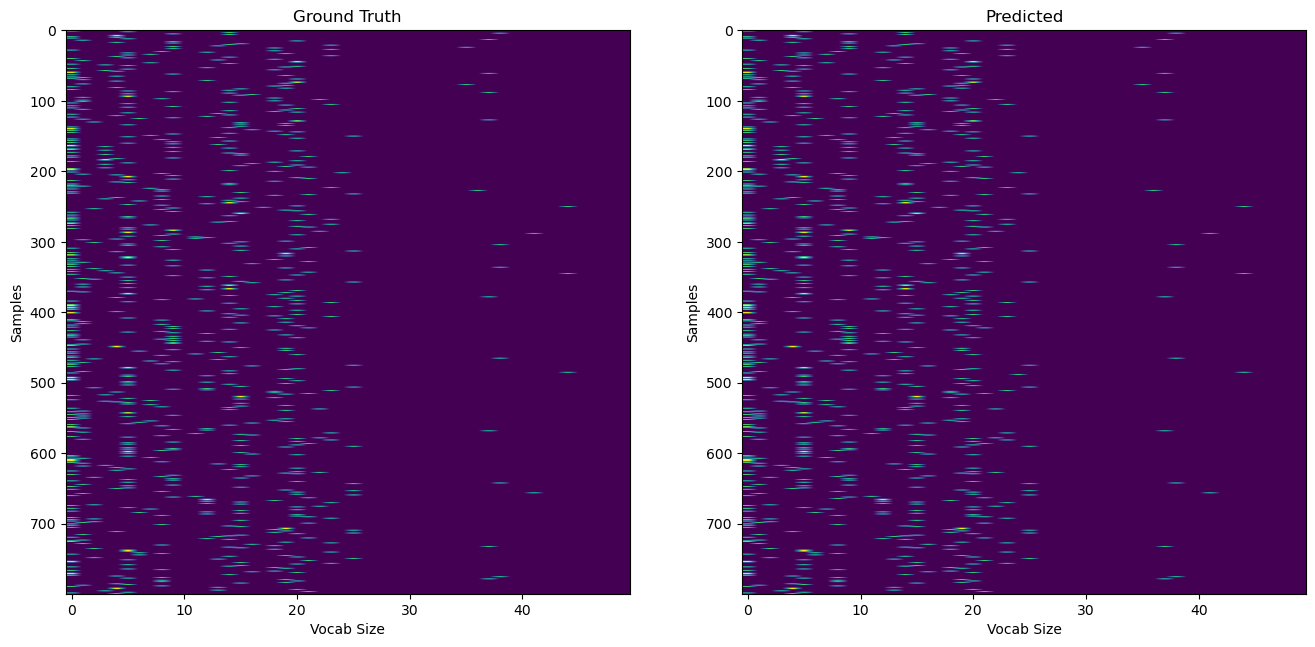
We see that the RFM model did pretty well. Now let’s look at the text that was actually generated.
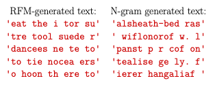
While we cannot draw conclusions on the models’ performances based on the generated text, we can still see that RFM generated text has actual words like “eat”, “the”, or “tool”. On the other hand, the N-gram generated text doesn’t produce actual words.
To assess the quality of our model, we calculate bleu scores and perplexity. Here are the results:
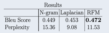
We see that the RFM has the highest bleu score and thus performs the best out of the three models. Indeed, in few-shot text generation, RFMs outperform N-grams and traditional kernels.
We also found out that kernles exhibit “double descent” which is a phenomenon that was thought to only be happening in DNNs. We also nothiced that RFMs exhibit stronger double descent than traditional kernels.
Conclusion
With the recent rise in popularity of language models like chatGPT, we wanted to compare text prediction between traditional neural networks and RFMs. By using 1984 by George Orwell as our training data and making predictions using an ngram model, a laplacian kernel and the RFM model separately, we were able to calculate Bleu score and perplexity and compare those scores for the three methods. By doing so, we were able to understand whether or not there exists methods better than classical neural networks for class prediction and generation. From our results, we found out that the RFM method has a higher Bleu score than the other methods which is a very interesting result. This innovative method has a lot of potential and applications. We saw how RFMs performed on text prediction but what about image classification? It would be very interesting to test the method on other datasets and understand where RFMs perform better.
Acknowledgements
A special thank you to Mikhail Belkin, Parthe Pandit for their help and guidance throughout this project.